For my first post, I’d like to focus on a very interesting intersection between financial economics and computer science I have been working on for the past semester while completing an undergraduate research project. This particular juncture is derivatives portfolio compression, a particularily important activity for financial firms looking to decrease their notional liabilities (due to recent regulatory obligations, a decrease in liabilities results in an increase in the flexibility institutions have to invest in capital.)

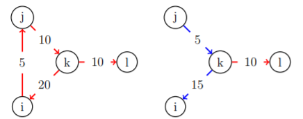
Portfolio compression is multilateral netting operation completed after a set of trades, which reduces counterparty risk (gross exposures between financial institutions) and maintains market risk (net exposures). Portfolio compression is unique from other netting operations because it reduces participant’s gross positions by tearing up redundant obiligations. In addition, portfolio compression can exploit multilateral netting opportunities without the participation of a Central Clearing Counterparty (CCP). Below is a stylized example of portfolio compression on a market consisting of four financial institutions:

My research this past semester has consisted creating an Open AI Gym environment that models this problem for the training of a reinforcement learning agent. The goal of this agent would be to derive an ofor compressing a set of derivatives contracts between groups of banks. Given the recent resurgence of financial regulation incentivizing actors within the financial sector to minimize their excess derivative contract notional, devising an artificial intellegence system to automatically minimize this excess over time is certainly a worthwhile endevour.

Problem Statement

Perhaps I should more concretely define the problem I intend to solve, before diving deeper into the OpenAI Gym I designed to acheive a solution.

First, we must define the following notation, a derivatives market can be modelled as consistenting the following elements:

1. A set of banks $B$ comprised of banks $(b_0,b_1,\dots b_n)$.
2. A set of timesteps $T = (0,1,2,3,4,5,\dots,n)$; each timestep $t \in T$ represents a week during which derivatives trading occurs.
3. A set of edges for every timestep $t$ that comprise a directed graph $G_t$, $E_t = (e_{t0},e_{t1}, \dots e_{tn})$; each edge $e_{ti} =(b_j,b_k)$ is of weight $w_t$, which represents an debt owed of $w$ million euros from bank $b_j$ to bank $b_k$ at timestep $t$.
4. An “arrival” of an edge is defined as one of two events:
   1. The origination of an edge $e_ti =(b_j,b_k)$ that did not exist in prior timesteps.
   2. The increase of the weight $w$ of an edge $e_ti$ that had existed in prior timesteps.
5. The total notional of a derivatives contract graph $G_t$ is equivalent to:

Where $w_t(b_i,b_j)$ is a function that returns the weight $w$ of the edge defined as a derivative contract relationship between bank $i$ and bank $j$ at timestep $t$.

Minimizing total notional at a given timestep $t$ is a solved problem, a paper that discusses the network simplex solution and how it effects a given derivatives contract network $G_t$ can be found here.

The precise problem that a intend to allow a reinforcement agent to learn how to solve is this:

If edges (derivative contracts) that arrive between banks due to a pattern determined by banks within a given financial system, can an agent to learn minimize notional excess over all periods? This can be formalized as solving for:

Where $w_t(b_i,b_j)$ is a function that returns the weight $w_t$ of the edge defined as a derivative contract relationship between bank $i$ and bank $j$ at timestep $t$.

Reinforcement Learning Problem

The corresponding reinforcement learning problem is very similar to the problem statement above, but with a few simplifications. They are outlined below:

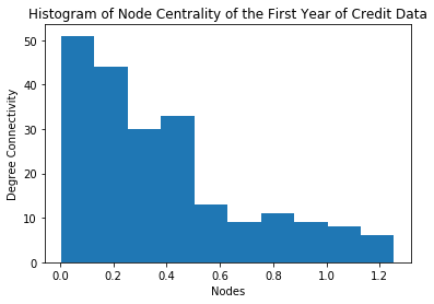
1. We will only be attempting to solve for the minimum amongst the top 10 most connected nodes, based on initial analysis, one can see that there are very few very connected nodes, so this is a fair simplification for the more general problem. A histogram is shown below:

1. For the early stages of this project, we will only aim to keep total notional below a certain percentage of what I define as counterfactual total notional, which is the total notional that would at time $t$ be observed given no action on all derivatives contract graphs $G_i$ for all $0 \geq i < t$, as of right now, this percentage of notional is set at 60%

Reward Structure

The reward structure of this problem is quite simple, our agent will recieve a reward of $-1$ for every time step it spends with total notional above the given threshold and positive 1 otherwise. Below is the “_get_reward” function in our OpenAi Gym environment.

def _get_reward(self):
        """Reward is given for each timestep below the is_compressed threshold."""
        if self.is_compressed:
            return 1
        else:
            return -1

Action Structure

As previously mentioned, minimizing the total notional amongst a set of banks $B$ and their respective edges $E$ while maintaining the amount owed from each bank to every other is a solved problem. It can be solved using the following linear programming problem:

Where $\hat{u}$ is a vector of all 1’s, $e’$ is the set of edges that would minimize total notional, $Q$ is an incidence matrix of our derivatives contract graph $G$ and $v$ is a vector representation of the total degree of each bank (which represents underlying value on each banks balance sheet).

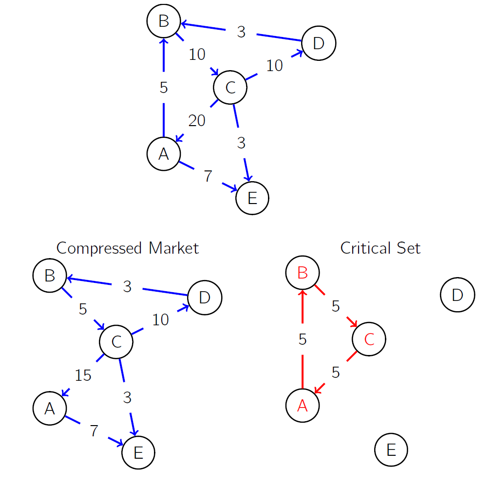
To figure out which cycles can be compressed in order achieve the minimum notional solution to the above linear programming problem, one could simply solve the problem, and subtract the solution of the problem from the original adjacency matrix. I denote this as the “critical adjacency matrix”. It is composed entirely of “critical cycles” or non-overlapping cycles that must be removed in order to completely conservatively compress a credit derivatives network graph. The actions that our agent can take are comprised of removing the first $i$ critical cycles, where $i$ is defined by the agent. The critical cycles are ordered by the decrease in notional excess, so removing the first $i$ critical cycles removes the $i$ critical cycles contributing most to unneccesarily high gross notional. If $n$ is the total number of critical cycles, action $n$ of our agent corresponds to subtracting all $n$ critical cycles from the current adjacency matrix (the adjacency matrix upon which the agent acts). Below is an example of a stylized derivatives contract market, its corresponding compressed market, and its corresponding “critical set”. The cycles of this graph are the critical cycles of the derivatives contract network.

Observation Structure

State Observations

THe observation structure of my agent is comprised of three components. The agent observes the state it exists in (the current derivatives contract market $G_t$), the actions it can take, and the reward it has recieved from its previous actions. After it makes a specific action, the agent sees an adjacency matrix repesenting derivatives contracts that have originated up to timestep $t$ between the top $m$ banks with the highest node centrality. As an adjacency matrix is a very noisy way to view and try to discern patterns within a derivatives contract graph, I have looked quite seriously into using the first $k$ singular values of the adjacency matrix to derive a rank $k$ representation of the adjacency matrix.

Action Observations

In addition, the agent observes the critical cycles of the adjacency matrix representing the culmination of derivatives contracts up to timestep $t$, these critical cycles are calculated by utilizing a conservative compression linear programming algorithm to find the graph that minimizes the notional excess of our derivatives contract graph. I then subtract this graph from the “current adjacency matrix” as described in “State Observations”. The cycles of this graph consist entirely of “critical cycles” or cycles that should be removed in order to miniminze excess notional in the derivatives contract graph. Given $n$ critical cycles, our agent can choose between action $ 0 < i \leq n$ where choosing action $i$ runs the following algorithm, as described in D’Errico and Roukny, for the first $i$ critical cycles (The critical cycles are ordered by the excess notional removed when they are compressed):

def compress_critical_cycle(ccycle,adj_matrix):
    path = ccycle['cycle']
    path_edges = [(path[i-1],path[i]) for i in range(1,len(path))]
    min_edge = min([adj_matrix[edge] for edge in path_edges])
    for edge in path_edges:
        adj_matrix[edge] = adj_matrix[edge] - min_edge
    return adj_matrix

Reward Observation

THh last observation to touch on is the observation that allows the agent to best discern how close it is to an optimal reward. Every timestep, our agent recieved information stating the current excess_percent. Which is the percent of counterfactual notional that is currently achieved by the current adjacency matrix. This is the same metric that will decide if an agent will recieve a reward of positive or negative 1 during a given timestep.

_get_state logic is displayed below:

    def _get_state(self):
        """Get the observation."""
        self.counterfactual_adj_matrix = self.counterfactual_adj_matrix + self.week_adj_matrices[self.curr_date]
        self.curr_adj_matrix = self.curr_adj_matrix + self.week_adj_matrices[self.curr_date]
        excess_percent = np.sum(self.curr_adj_matrix)/np.sum(self.counterfactual_adj_matrix)
        compress_res = compress_data(self.curr_adj_matrix)
        critical_matrix = compress_res["critical_matrix"]
        compressed_matrix = self.curr_adj_matrix - critical_matrix
        self.ccycles = critical_list_from_matrix(critical_matrix)
        return dict({"curr_adj_matrix":normalize_matrix(self.curr_adj_matrix),
                    "compressed_matrix":normalize_matrix(compressed_matrix),
                    "excess_percent":excess_percent})

Results

Unfortunately, due to the time constraints of the semester, I was unable to build a deep learning agent to train within in the OpenAI Gym I intended to build. However, I was able to build the gym environment and to test various policies on it. For these tests, I used the 10 most connected banks and I used the timesteps of the 57 weeks from January 5th, 1999 to Febuary 8th, 2000. I tested 3 policies for 100 episodes:

1. A policy in which the agent compresses all critical cycles left in the derivatives market’s graph. At every timestep, this policy calculates the critical cycles of the graph and compresses all of them.
2. A policy in which the agent compresses 500 critical cycles left in the derivatives market’s graph. At every timestep, this policy calculates the critical cycles of the graph and compresses all of them.
3. A policy in which the agent compresses a random number of cycles.

Below are the eliminate notional at each time step by each policy. The minimum notional achieved by the random policy uses an average of 100 random polices. The red line, denoted “minimum notional” calculated as the the minimum notional achieved if at the last time step, the algorithm described in Roukny and D’Errico is run. This is the minimum possible excess percent utilizing conservative compression. A compression policy can be evaluated by its distance towards this metric, which for this time interval, and this number of banks is about 44%.

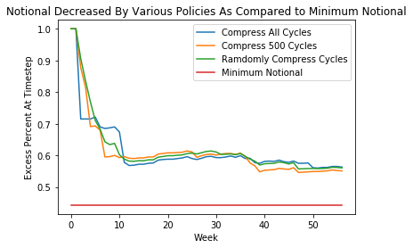
While it would be intuitive that compressing all cycles at every timestep decreases notional significantly, the figure above shows that this is not the case. In fact, there is a great deal of room between the minimum notional (44%) and the resulting notional from the three policies analyzed, which seem to have equivalent success. This “optimization gap” is nontrivial, as it leaves about 13 billion euros uncompressed in the european credit derivatives market. The lower level achieved by compressing only 500 cycles each timestep seems to suggest the presence of a “happy medium” between compressing all cycles and compressing no cycles that yields lower excess notional at the end of each episode (one round of compressing at every time step). This “happy medium” could likely be found by a reinforcement learning agent.

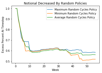
It is also noteworthy that there is a great deal of variation in results amongst the random agent’s 100 episodes. Below is a plot denoting the random agents average performance, its maximum performance, and its minimum performance.

Next Steps

1. Build a deep learning agent trained with my model, as of right now the cross entropy agent from the OpenAI Gym package that I am using has quite poor performance; I made this gym enviroment to test architectures with stronger pattern recognition abilities, and I certainly would like to test my environment on such architectures.

2. I have been playing quite a bit with the idea of sending the reinforcement learning agent information about only portions of the singular value decompisition of the “current state adjacency matrix” (such as its SVD). This would help accentuate patterns within the adjacency matrix amongst banks with very distinct trading patterns. Once I am able to begin to work more seriously on using a deep learning architecture for policy discovery this will definitly be the first mutation of the very noisy adjacency matrix that I will try.

Codebase

The Open AI Gym I built, and the random agents I used to test it is all public here on my github.